Map the IO

IO Mapping establishes the program interface between the workstation's physical IO and the internal variables used throughout the control application. In this tutorial, we will build that interface from the completed IO Schedule and organize the mapping logic around it.

We will map the inputs first. This process begins by creating a MapInputs program space and then adding it to the workstation program MainTask so it becomes part of the cyclic control program.

We will then map the physical inputs to their corresponding internal variables. As we do, we will review what condition each mapped input should represent when it is TRUE and program the mapping accordingly.

We will prepare to map the outputs in much the same way. We will create a MapOutputs program space and then add it to the workstation program MainTask so it becomes part of the cyclic control program.

We will then map the internal output commands to their corresponding physical outputs. The mapping will remain intentionally simple, with the workstation control logic determining what should be commanded and MapOutputs transferring those commands to the physical IO.

This tutorial is using CODESYS as the program development environment. IO Mapping presents the same set of advantages regardless of the PLC platform or programming environment in use.

Ordinary programmers often use the particular IO hardware and addressing native to an installation. This means that any time an input is moved to another terminal and therefore another address, the programmer is faced with having to comb the entire program for references to the old location. IO Mapping eliminates that need by placing a defined program interface between the physical IO and the control logic that uses it.

IO Mapping also makes troubleshooting easier. With an orderly naming convention such as Input001, Input002, Input003, and so on, a technician looking for Input034 can quickly locate it in the mapping logic and observe the state and address of the corresponding physical input. Without that organization, locating the same signal may first require knowing or tracing whatever hardware-specific physical address was assigned to it.

These advantages may seem minor when considered individually, but they become significant over the life of a control program. They are practical, field-tested benefits of IO Mapping that shorten development time and provide real uptime effects during troubleshooting, modification, and long-term maintenance events.

We begin the workstation input mapping by creating a Global Variable List beneath the CODESYS Application. The mapped input variables will be used throughout the control program rather than belonging to any one program POU, so we create a Global Variable List named GVL_IO to contain them.

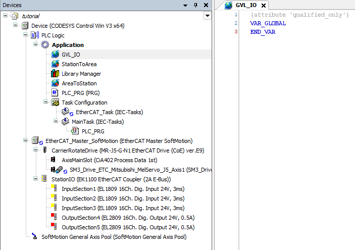
Returning to the Discrete Inputs worksheet of the IO Schedule, we see that the workstation has 48 physical input points. We therefore create 48 individual Boolean variables in GVL_IO, using the established Input001 through Input048 naming convention.

We deliberately declare these as individual variables rather than as elements of an array. Although this requires more initial declaration work, it allows each mapped input to carry its own description wherever that variable is used in the control program. This is an important distinction in CODESYS, where the individual elements of a Boolean array do not carry separate declaration descriptions throughout the program.

These booleans are declared as unqualified global variables. This allows us to use them programmatically as they appear, such as Input034 rather than GVL_IO.Input034. One downside of this is that the Input001 through Input048 names can be declared again in some other context. This can lead to real confusion and wasted time for future troubleshooters... so don't do that. We initially set each variable to FALSE and identify it as a Spare Input.

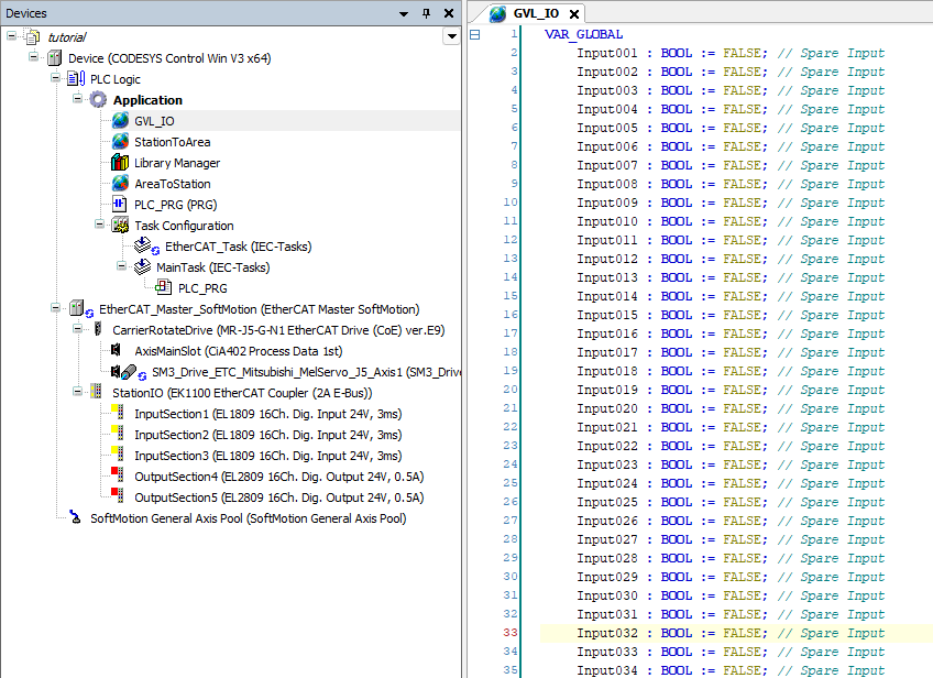
We next return to the Discrete Inputs worksheet of the IO Schedule and replace the temporary Spare Input description for each assigned input with the description developed for that input. The unused input points remain identified as Spare Input. This completes the initial definition of the mapped input variables before we begin using them in the control program.

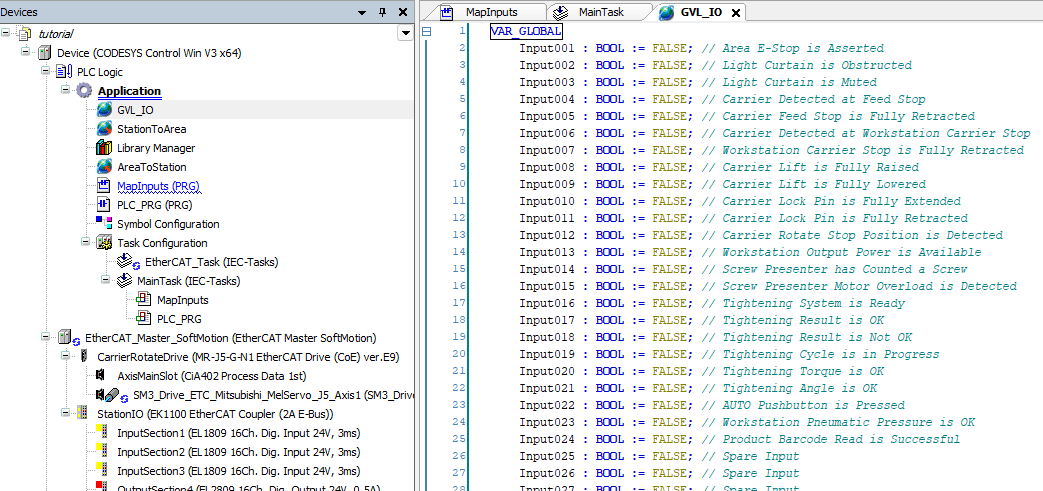
The next preparation step for mapping the inputs is to create the Ladder section that will contain the rungs used to perform the actual mapping. In some programming environments, this may simply be another Ladder routine or program section. In CODESYS, we create a separate PROGRAM POU using Ladder Logic.

The input mapping program is always placed first in the workstation control-program scan so the mapped input variables are established before any workstation control logic evaluates them later in the scan. It should remain first as the application grows, preserving a predictable scan structure in which the control program always begins from the current mapped state of the physical inputs.

To create the input mapping program in CODESYS, we add a new POU to the Application. We name it MapInputs, select Program as the POU type, and choose Ladder (LD2) as the implementation language. This gives us a separate Ladder program that can be placed first in MainTask and used exclusively for the workstation input mapping.

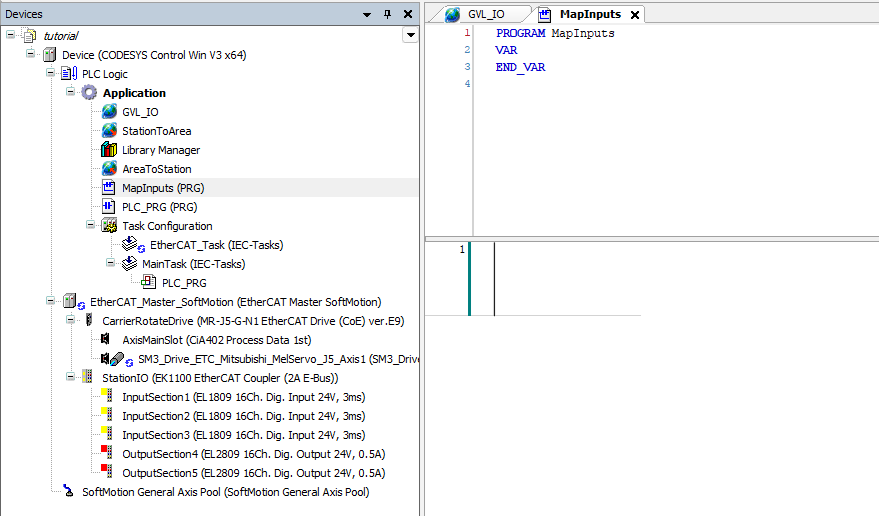
Adding MapInputs beneath the Application creates the Ladder program, but does not cause it to execute. In CODESYS, program execution is established through the task configuration. We therefore add MapInputs to MainTask.

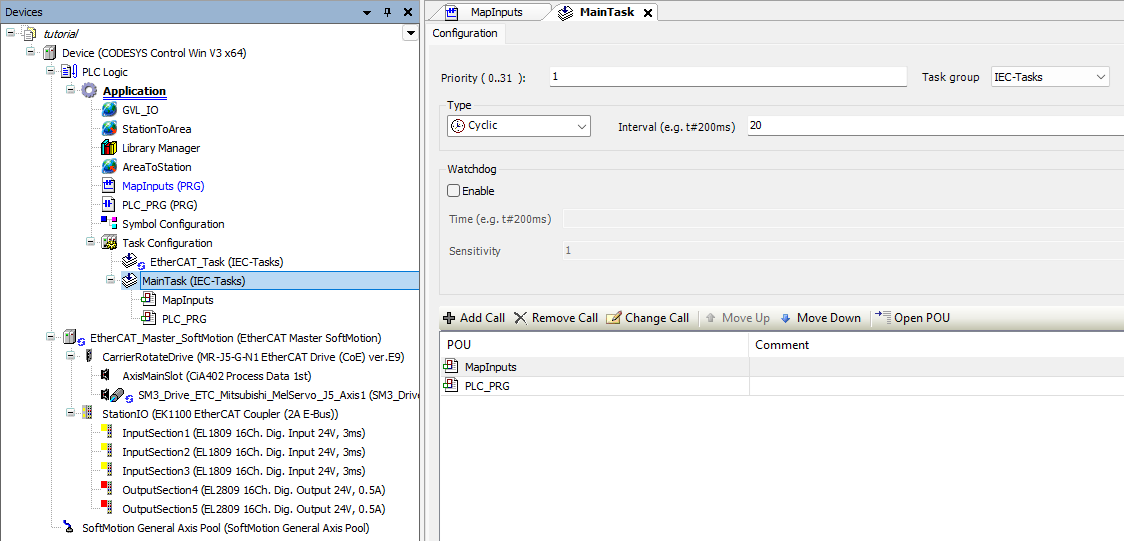
The last preparation step is to place MapInputs first in the scan order. We double-click MainTask to open its configuration. The program-call list contains the default PLC_PRG and our MapInputs program. Because the calls execute from top to bottom, we use Move Up to place MapInputs first, making it the first workstation program executed during each cyclic scan.

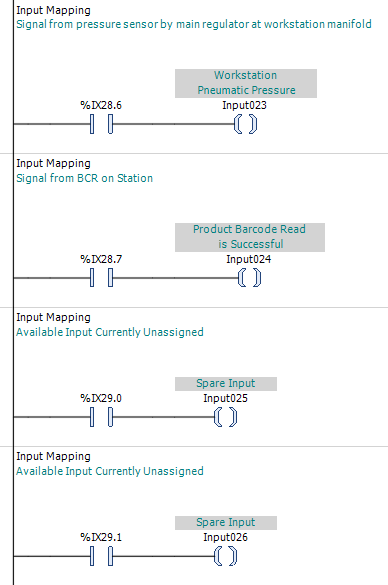
With the mapped variables and MapInputs program prepared, the actual input mapping is straightforward. Working through the Discrete Inputs worksheet of the IO Schedule in order, we use the physical CODESYS Address as the input condition on a Ladder rung and the corresponding Input Name variable as the output of that rung.

The mapping does not necessarily preserve the electrical sense of the physical signal. For each input, the PLC Pro decides what condition will be most useful for the corresponding Input Name to represent when it is TRUE. The Description in the IO Schedule records that meaning, and the mapping rung is programmed so the mapped variable becomes TRUE when that described condition exists.

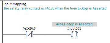
We begin with Input001, described in the IO Schedule as Area E-Stop is Asserted. What we want the mapped variable to tell us is when to put the workstation into E-Stop Mode. The safety relay contact supplying the physical input is energized when the safety circuit is healthy and drops out when E-Stop is asserted, so the physical signal has the opposite sense from the condition we want Input001 to represent. We therefore use the physical input as a negated condition in the mapping rung so Input001 becomes TRUE when the Area E-Stop is asserted.

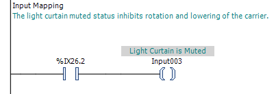
Input003 provides an example in which no inversion is required. What we want to know is when the light curtain is muted, and the physical muting-status signal is TRUE while muting is active. We therefore describe Input003 as Light Curtain is Muted and map the physical input directly to it. When the physical input is TRUE, Input003 is TRUE.

We continue through the IO Schedule in the same manner, mapping each assigned physical input to its corresponding Input Name. We also map several currently unused points in the second half of InputSection2 and leave their descriptions as Spare Input. Adding IO during commissioning is common, and having a few spare points already mapped gives us immediately available program interfaces when that occurs.

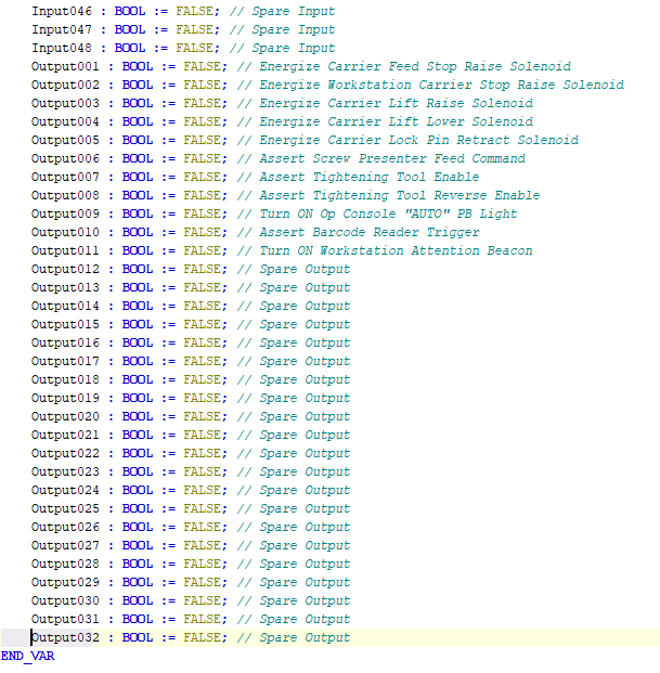
Preparing to map the workstation outputs follows much the same pattern we used for the inputs. We begin with the Discrete Outputs worksheet of the IO Schedule and add the required mapped output variables to the existing GVL_IO Global Variable List.

The workstation has 32 physical output points, so we create 32 individual Boolean variables using the established Output001 through Output032 naming convention. As with the mapped inputs, these are unqualified global variables and are initially set to FALSE.

We then transfer the descriptions from the Discrete Outputs worksheet to the corresponding assigned output variables. Unused points remain identified as Spare Output. This gives each mapped output the same readily available identification in the control program that we established for the mapped inputs.

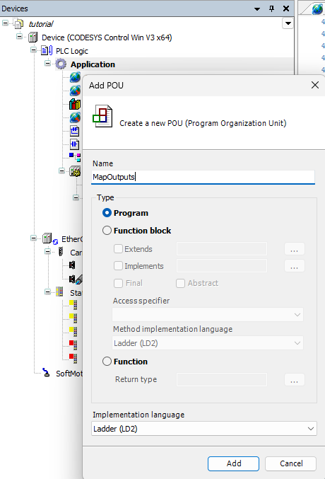
We next create a separate PROGRAM POU named MapOutputs beneath the Application, using Ladder (LD2) as the implementation language. This creates the program that will contain the output-mapping rungs, but does not cause it to execute. Execution is established separately by adding MapOutputs to MainTask.

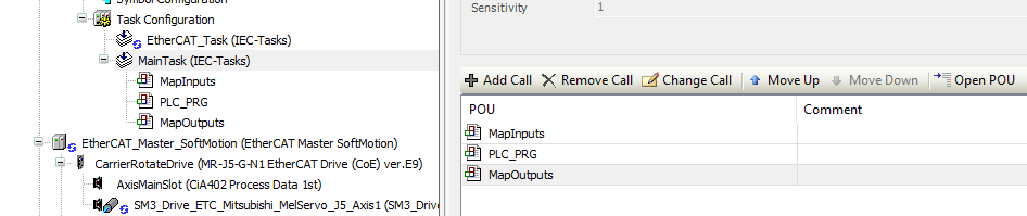
We then add MapOutputs to MainTask. This causes the program to execute as part of the workstation's cyclic control scan.

The output mapping program must execute after the workstation control logic has determined the commanded state of the mapped outputs. We therefore verify that MapOutputs is last in the MainTask program-call order. CODESYS has placed the newly added program call at the bottom of the list by default, so no repositioning is required in this case.

The resulting scan structure is the pattern we will preserve as the application grows: MapInputs first, the workstation control programs between them, and MapOutputs last.

With the mapped output variables and MapOutputs program prepared, we can begin connecting the workstation's internal output commands to the physical outputs identified in the Discrete Outputs worksheet of the IO Schedule.

Output mapping reverses the direction we used for the inputs. The mapped Output Name is used as the condition on the Ladder rung, and the corresponding physical CODESYS Address is used as the output of that rung. The workstation control logic therefore commands the mapped output variable, while MapOutputs applies that command to the physical output.

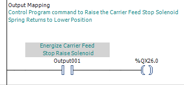
We begin with Output001, described in the IO Schedule as Energize Carrier Feed Stop Raise Solenoid. When the control program makes Output001 TRUE, the mapping rung energizes physical output %QX26.0, applying power to the Carrier Feed Stop raise solenoid. When Output001 is FALSE, the physical output is de-energized and the spring returns the stop to its lowered position.

This direct one-to-one mapping is typical of PLC Pro programs. MapOutputs does not normally contain the control decisions associated with the equipment. Each mapped output command is transferred independently to its corresponding physical output.

The Carrier Lift provides a good example. Output003 energizes the Carrier Lift raise solenoid, while Output004 energizes the Carrier Lift lower solenoid. Although those two solenoids must not be energized at the same time, that mutual exclusion is handled in the workstation control logic that develops the two mapped output commands. MapOutputs simply transfers the resulting command states to the corresponding physical outputs.

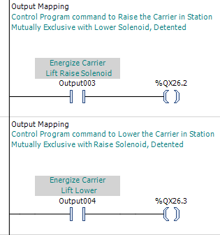
We continue through the Discrete Outputs worksheet in the same manner, mapping each assigned Output Name directly to its corresponding physical CODESYS Address. The mapping remains intentionally simple; the workstation control logic determines when each command should be asserted, and MapOutputs transfers that resulting command to the physical output.

As we work through the output mapping, we also continue developing the IO Schedule. The IO Schedule is a PLC Pro working document, and its content is not fixed simply because the original IO has been identified. When the programming work reveals information that will be useful later, we add it. In this case, details such as spring-return behavior and detented valves are added to the Notes column as their importance becomes apparent.

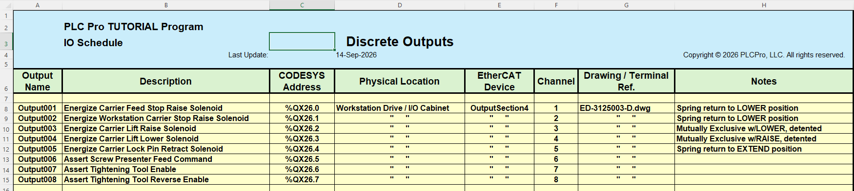
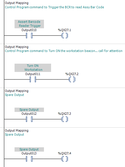
As we did with the inputs, we also map several currently unused physical output points and leave their descriptions as Spare Output. Adding IO during commissioning is common, and having available points already mapped gives us immediately usable program interfaces when that occurs.