Develop the IO Schedule

A PLC Pro IO Schedule is a spreadsheet that records the pertinent details of each input or output resident in or referenced and used by the control program to interface with and control the workstation equipment and activities. Having all of this detail in one organized, searchable document is extremely useful, and in many ways essential, for rapid and accurate control program development.

We begin by developing the Discrete Inputs portion of the IO Schedule from the electrical drawings. This establishes the worksheet structure, the local input naming convention, the descriptions used by the program, and the physical and drawing-reference information available for each input.

We then develop the Discrete Outputs portion of the IO Schedule using the same electrical design information. Assigned output points and available spares are recorded so the outputs available to the workstation program are identified before equipment logic is developed.

The workstation servo drive introduces an intelligent-device interface that cannot be completely defined from the electrical drawings alone. We establish the required CODESYS EtherCAT and SoftMotion configuration, add the servo drive to the project, and use the drive documentation together with the CODESYS configuration to document its control, command, status, and feedback data in the IO Schedule.

Once the CODESYS EtherCAT structure is established, we add the discrete IO hardware identified earlier from the electrical drawings. The actual terminal mappings then provide the CODESYS addresses needed to complete the Discrete Inputs and Discrete Outputs portions of the IO Schedule.

Finally, we establish the communications interface between the workstation and the Area PLC. The required data exchange is implemented using CODESYS network variables over UDP and documented in the IO Schedule using the qualified CODESYS variable names, datatypes, default values, descriptions, and direction of communication.

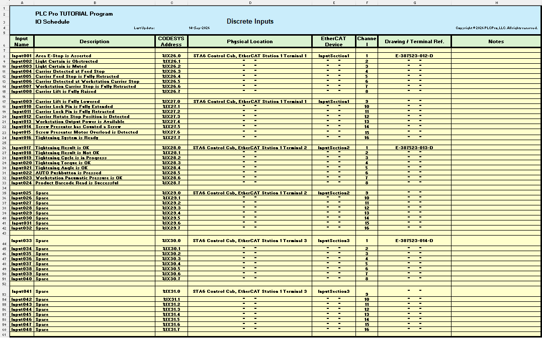
We begin the workstation IO Schedule by creating a blank Discrete Inputs worksheet. This worksheet simply gives us a place to begin recording the information we will need to track the discrete inputs available to the control program. It's OK to miss something or get something wrong here. The IO Schedule will change in both content and structure as we examine the full system design and develop a more complete understanding of what information is important to have readily available during program development.

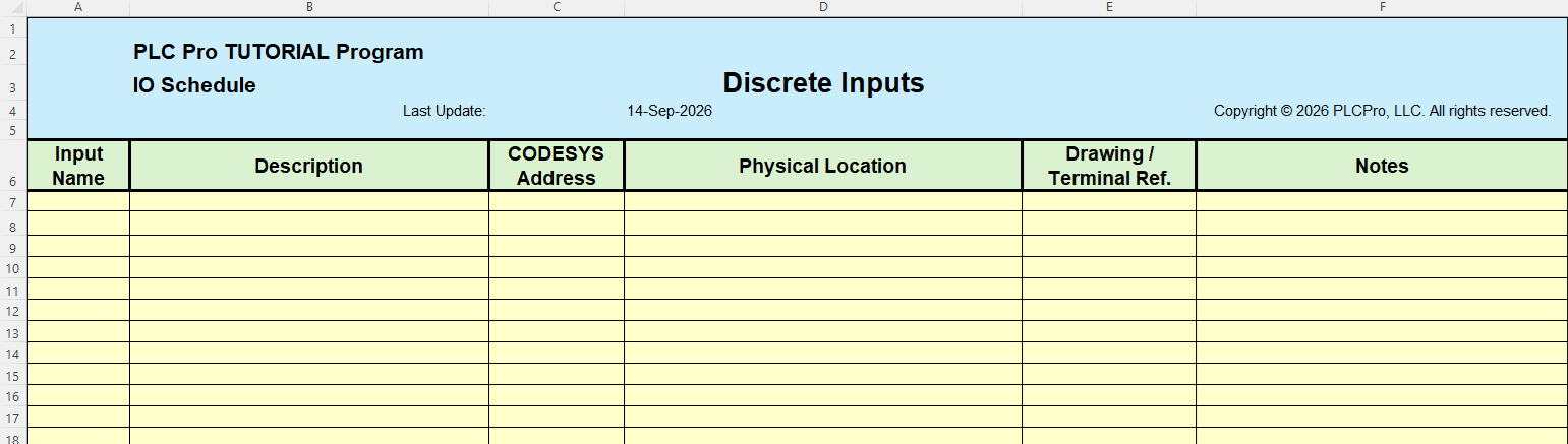
For now, we have chosen to record an Input Name, Description, CODESYS Address, Physical Location, Drawing / Terminal Ref., and Notes for each input. These headings represent our initial judgment about information that may be useful as the control program is developed. We will revise them if experience with the workstation shows that something different would be more useful.

Most of the fields shown on the worksheet are self-explanatory. Input Name, however, deserves some explanation. PLC Pro programs use IO Mapping, and each physical input therefore needs a local program variable to which it can be mapped. The Input Name is the name assigned to that local variable. IO Mapping is explored in more detail in the sections describing input and output mapping.

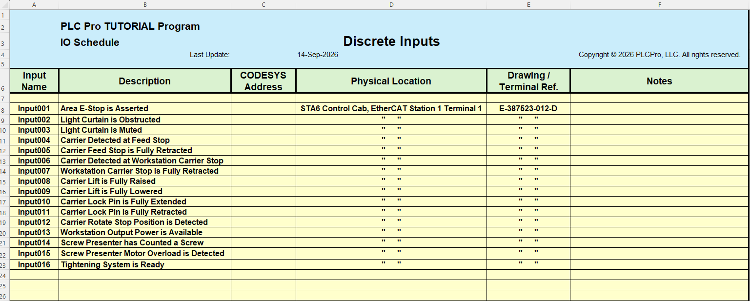
We will keep the local input naming convention simple. Each mapped input will be assigned a unique sequential name beginning with "Input": Input001, Input002, Input003, and so on. When one of these names appears in the control program, the same name provides a quick way to locate that input and its associated information in the IO Schedule.

The electrical drawing also identifies the physical devices connected to the PLC inputs. We use that information to construct the input descriptions. The PLC Pro naming convention is to describe what each mapped Input Name means to the control program when it is TRUE.

The electrical drawing also provides the physical-location and drawing-reference information needed for the IO Schedule. We record that information as the inputs are added.

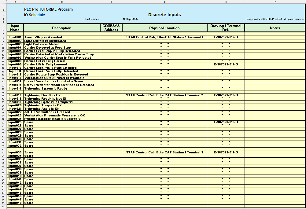
Continuing through the electrical drawings, we find two additional 16-point input terminals. We add all of their input points to the IO Schedule, entering descriptions for the assigned inputs and identifying the unused points as Spare. This gives us a complete first pass at the discrete inputs shown on the electrical drawings.

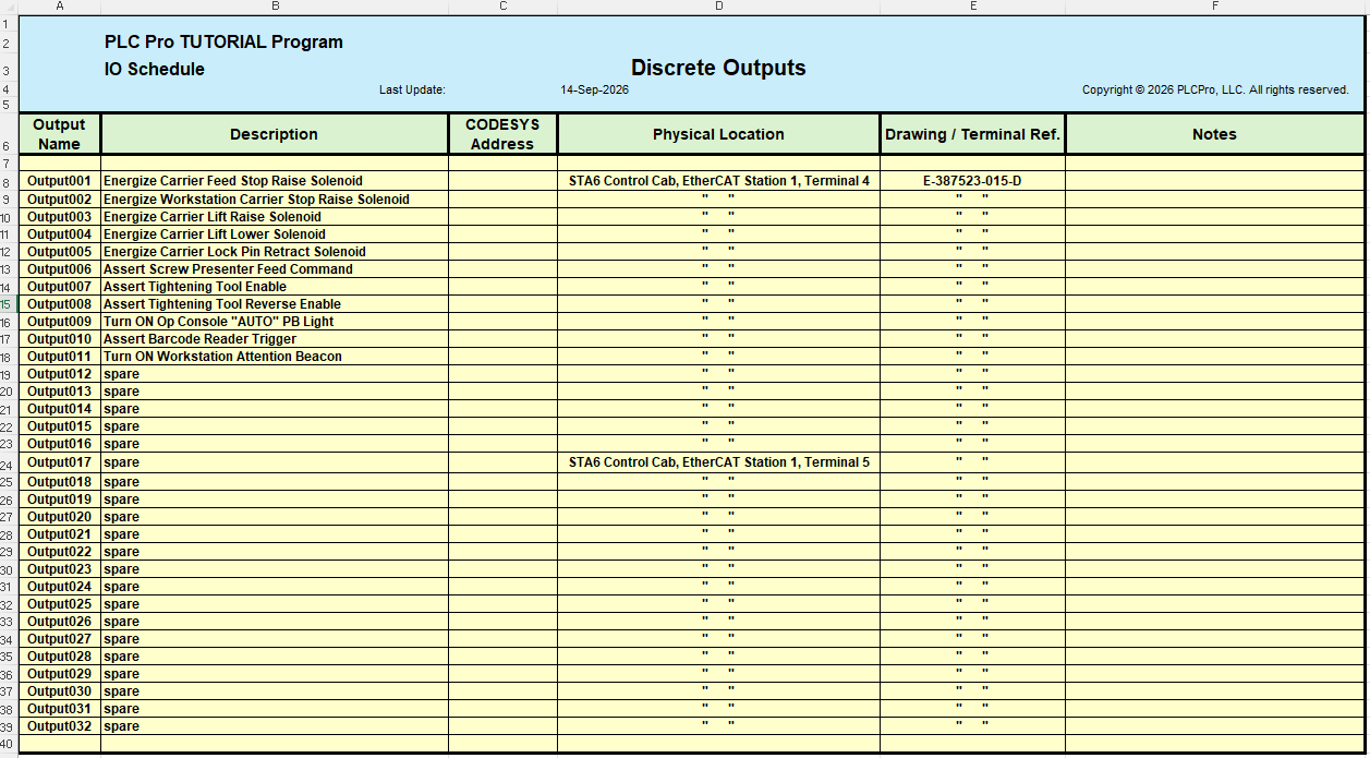
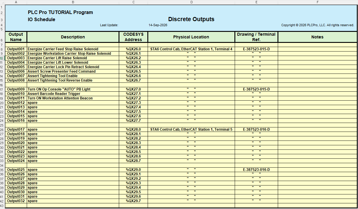
We use the same basic procedure for the discrete outputs. Reviewing the electrical drawings identifies two 16-point output terminals. We add each output point to a Discrete Outputs worksheet, enter descriptions for the assigned outputs, and identify the unused points as Spare.

The electrical drawings also identify a Mitsubishi MR-J5-G-N1 EtherCAT servo drive for the workstation rotary table. At this point, the only hardwired interface shown between the control system and the drive is the safety-stop circuit. The normal operating interface to the drive will therefore need to be established next as we continue developing the IO Schedule.

To establish the normal operating interface to the drive, we now begin developing the CODESYS project. We create a new Standard project for the workstation. The standard project provides the initial application, PLC_PRG, and a MainTask with PLC_PRG assigned to it. This gives us the basic program structure from which we can begin adding the EtherCAT hardware required by the workstation.

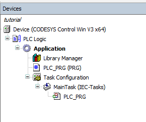
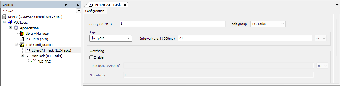
The MR-J5-G-N1 servo drive communicates with the control system through EtherCAT. According to the CODESYS EtherCAT documentation, EtherCAT process data is exchanged with the physical bus in a designated bus-cycle task. The standard project already includes MainTask for execution of the IEC control program, so we create a separate cyclic task named EtherCAT_Task for the EtherCAT communication.

The EtherCAT_Task is created with configuration values appropriate to the application. The required task interval, priority, watchdog settings, and other execution parameters should be determined from the needs of the application and the applicable CODESYS and device documentation.

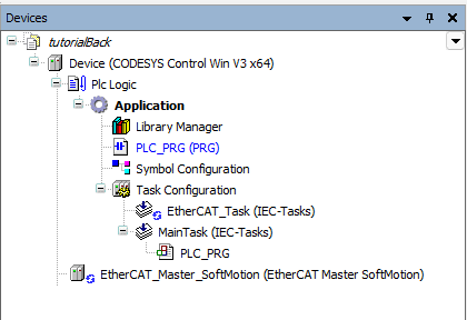
We next add a device at the Device level of the CODESYS project. Under the available Fieldbuses, the EtherCAT options include EtherCAT Master SoftMotion. We select this master because the workstation uses the MR-J5-G-N1 servo drive and we need CODESYS SoftMotion to operate the drive.

Once added to the project as above, double-click the EtherCAT Master SoftMotion to open its configuration dialog. The EtherCAT master must be associated with the network interface card (NIC) that will be used for EtherCAT communication. The Select... tool displays the available network adapters and can often be used to select the appropriate NIC and assign its MAC address to the master.

With the EtherCAT Master SoftMotion installed and configured, we next add the Mitsubishi MR-J5-G-N1 servo drive beneath the master as an EtherCAT device. If the drive model does not appear in the available device list, download the appropriate EtherCAT device-description (ESI) files from the drive manufacturer and install them in the CODESYS Device Repository. Then you can return to the Add Device dialog and select the drive from the list.

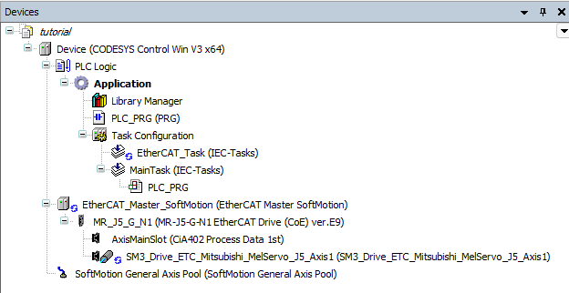
After the drive is added, we rename it CarrierRotateDrive to identify the equipment function it serves in the workstation. This is done by using the "Refactoring" option after right-clicking the installed drive.

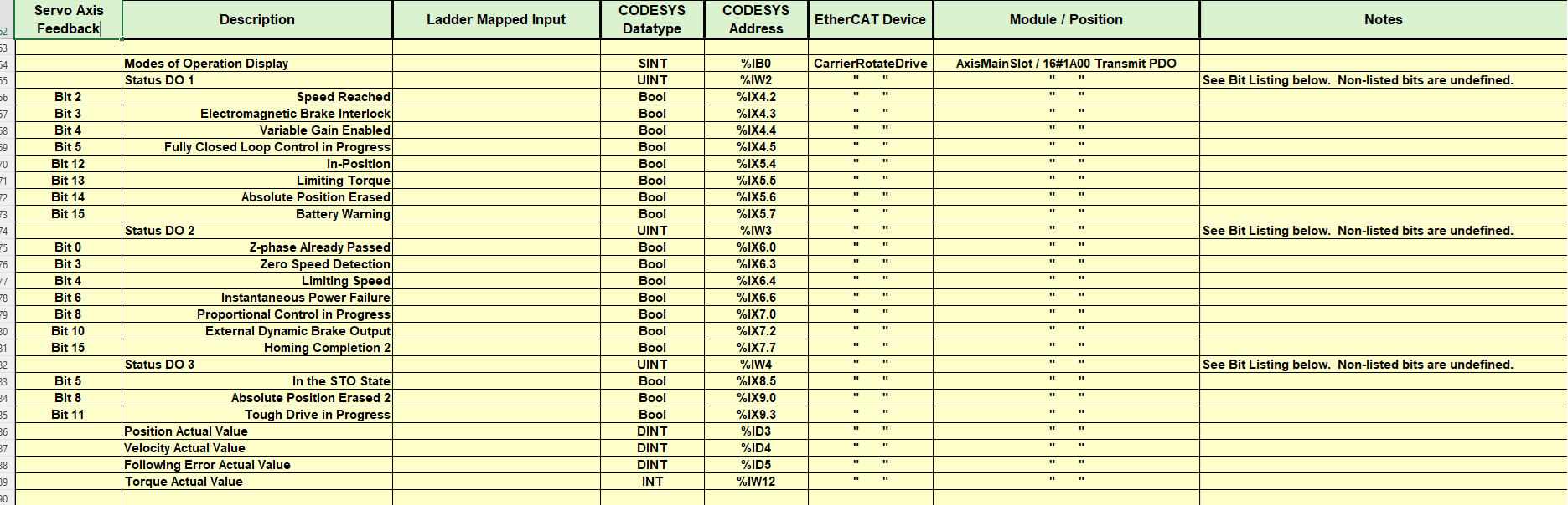
With CarrierRotateDrive now installed in the CODESYS project, we can begin completing the servo-drive portion of the IO Schedule. The drive configuration provides CODESYS-specific information that we could not establish from the electrical drawings or drive documentation alone, including the EtherCAT device name, datatype, and CODESYS address for each process-data item.

The first drive interface of interest from a programming standpoint is the Drive Control Word. This 16-bit output word contains the individual control bits used by the program to manage the operating state of the servo drive. We therefore begin the servo-drive portion of the IO Schedule by identifying the Control Word and the function of each of its bits.

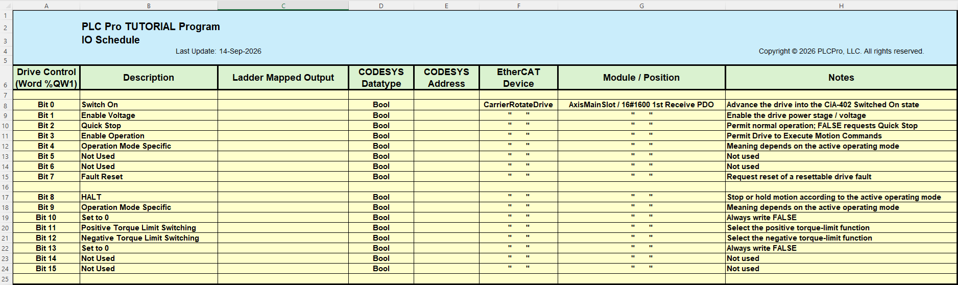
At this point, we can already populate much of the Drive Control section of the IO Schedule. The Mitsubishi documentation identifies the function of each Control Word bit, while information available in the CODESYS project identifies properties such as the datatype, EtherCAT device, and module position. The CODESYS addresses and any ladder-mapped outputs have not yet been established.

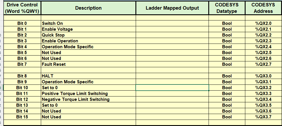
Next, we open the AxisMainSlot Module IO Mapping. Here CODESYS shows the Controlword at %QW1 and provides the individual address assigned to each of its bits. We use these addresses to complete the CODESYS Address column of the IO Schedule.

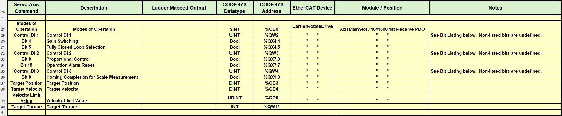
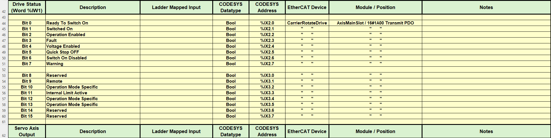
From here, we continue through the remaining servo-drive process data using the same procedure. The Mitsubishi documentation identifies the purpose and meaning of each item, while the corresponding CODESYS axis-object mapping provides the datatype and CODESYS address. We use those two sources together to complete the remaining servo-drive entries in the IO Schedule.

The discrete inputs and outputs identified earlier from the electrical drawings now need to be represented by the actual IO hardware in the CODESYS project. With the EtherCAT Master SoftMotion established, we add the workstation EtherCAT coupler beneath it, then add the input and output terminals in their installed order. After the devices are added, we rename the coupler and each terminal to make their purpose and physical grouping clear in the CODESYS project.

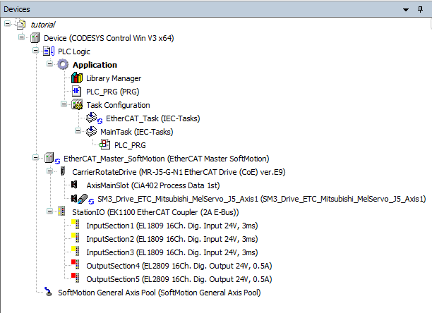
With the workstation EtherCAT IO now installed in the CODESYS project, the addresses assigned to each discrete input and output are available from the terminal IO mappings. We use those mappings to complete the CODESYS Address columns in the Discrete Inputs and Discrete Outputs worksheets of the IO Schedule.

The workstation does not operate entirely on its own. It must exchange information with the Area Controller to coordinate its operation with the surrounding production area. This will include requests for disposition for carriers entering the station, and later reporting on station activity.

Before implementing that communication, the information to be exchanged must be defined. In an actual installation, this will normally be coordinated with the person or group responsible for the Area Controller and documented as an interface specification identifying the data required in each direction, its datatype, and its intended meaning.

Communication with the Area Controller will use CODESYS network variables transmitted over UDP on the Ethernet network. CODESYS implements network-variable communication using separate Sender and Receiver lists, so the two-way exchange with the Area Controller requires one list for each direction.

We begin with the data the workstation will send by right-clicking the Application and selecting Add Object → Network Variable List (Sender). We name this list StationToArea and select UDP as the network type. Using Settings..., we enter the UDP port and the broadcast address appropriate for the Ethernet network used by the workstation and Area Controller.

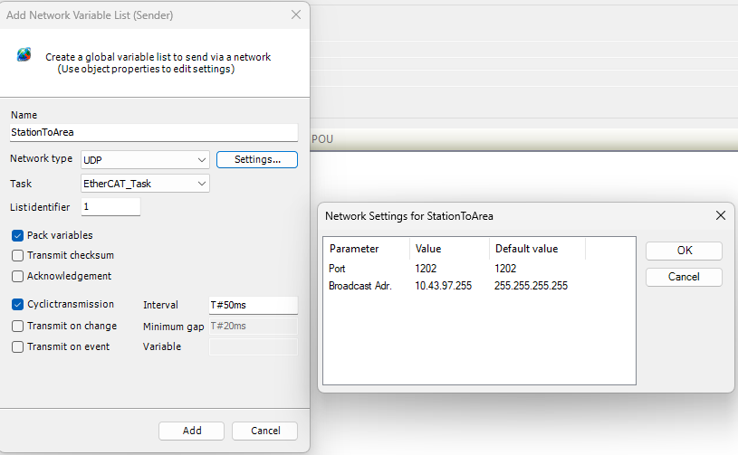
After the StationToArea sender is added, CODESYS opens its global variable list. Using the interface specification, we enter the variables the workstation will transmit to the Area Controller, including the required name, datatype, default value, and description for each value.

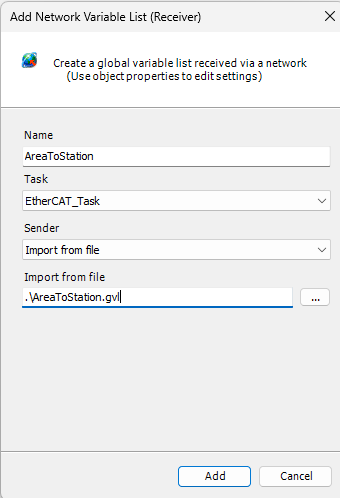
We next add a Network Variable List (Receiver) beneath the Application and name it AreaToStation. The variables to be received are already defined in the Area Controller program and exported from that project as a .gvl file. When creating the receiver, we identify that file so CODESYS can use the exported variable definition for the AreaToStation exchange.

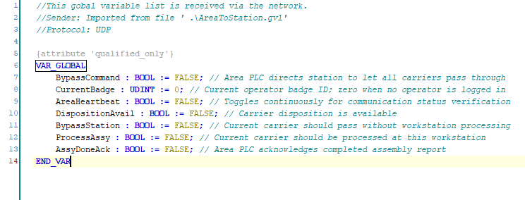
After the receiver is created, CODESYS displays the imported AreaToStation global variable list. The list now contains the variables defined by the Area Controller project, including their names, datatypes, default values, and descriptions, and identifies UDP as the protocol used for the exchange.

We document the Area Controller exchange on its own IO Schedule worksheet. Unlike physical IO, these values are CODESYS network variables rather than addressed input or output points, so the schedule records the qualified CODESYS variable name used by the program along with each variable's datatype, default value, description, and direction of communication.

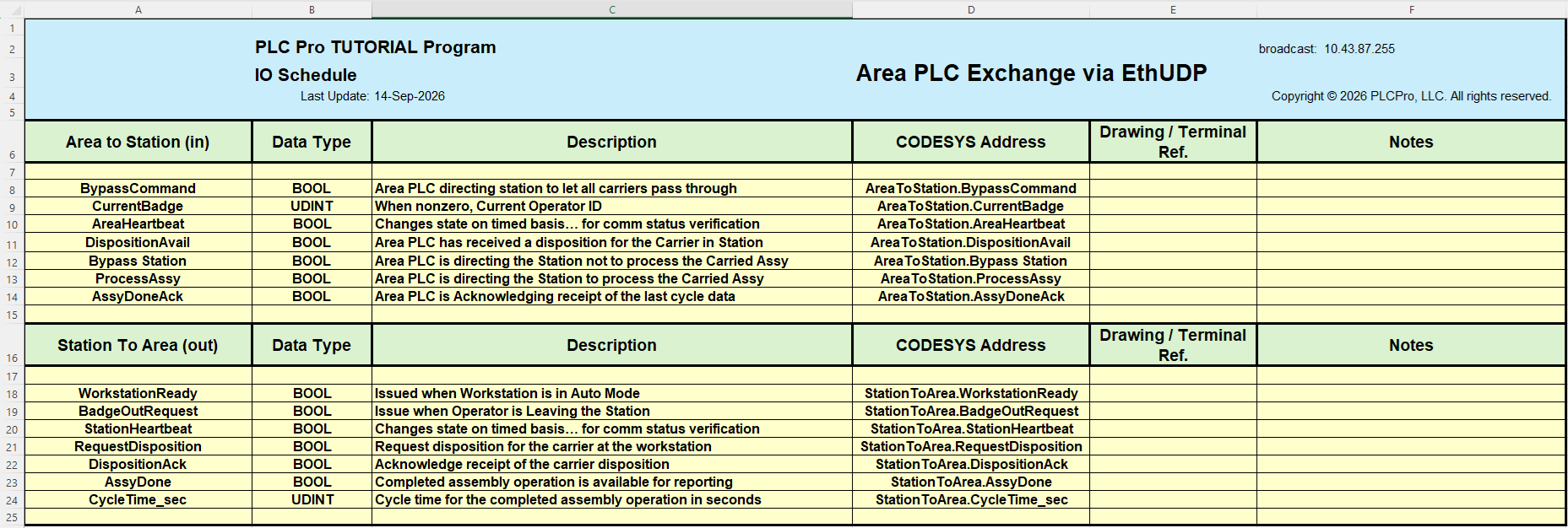
This completes our first pass through the IO Schedule. We have documented the discrete inputs and outputs, servo-drive control and feedback data, and the two-way Area Controller interface currently available to the workstation program. The IO Schedule will continue to evolve as program development identifies additional information, naming changes, or interface requirements that need to be recorded.